The purpose of Lab 9 was to perform mapping on an environment in the lab using a PID controller. Since I was
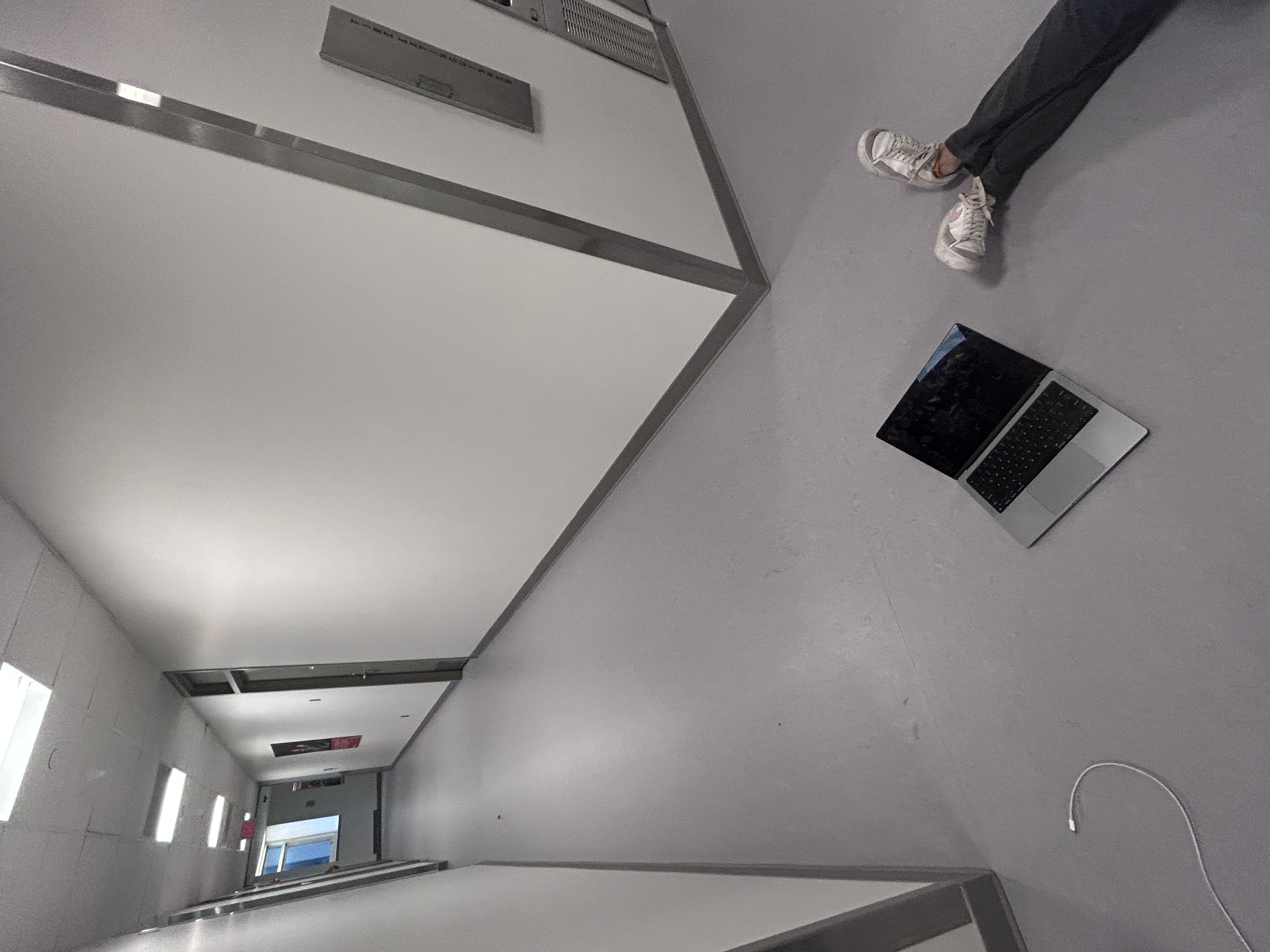
running short on time I did the mappings in a hallway in Rhodes Hall.
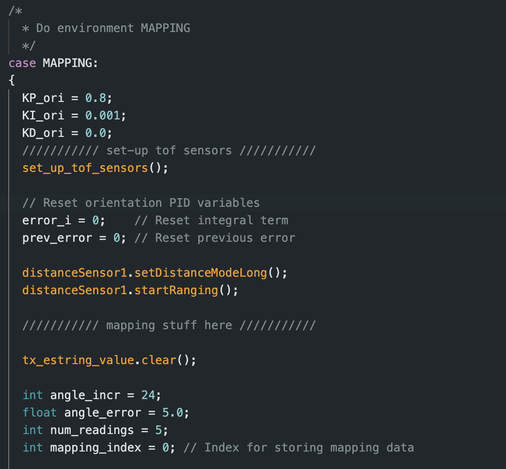
PID Controller
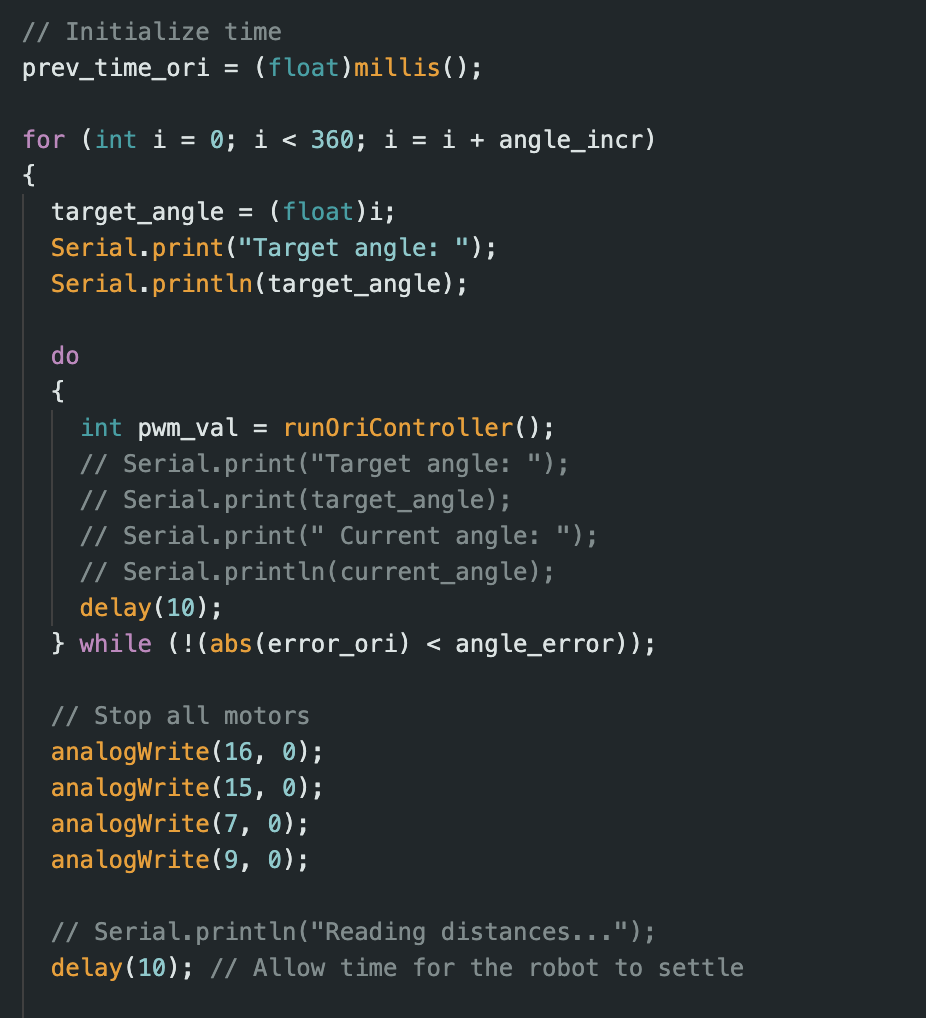
I chose to use option 2 from the lab handout for my orientation control. I set a fixed angle
incremet of 24 degrees that looped through the angles from 0 degrees to 360 degrees using my PID orientation
control loop. To achieve this I set up a new case in my arduino code called MAPPING. The robot systematically
rotates in increments of 24 degrees, using a PID
controller with preset gain values of KP=0.8, KI=0.001, KD=0 that I found via calibration, to accurately achieve
each target angle within a 5-degree
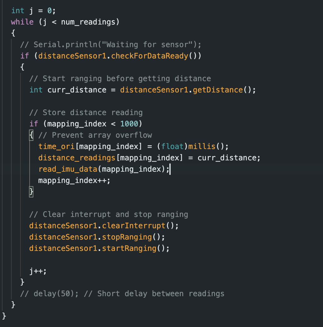
error threshold. At each position, the robot collects 5 distance readings along with timestamps and
orientation data from the IMU. I got a total of 45 datapoints over 9 angles. Once the full rotation is complete,
all collected data points: time,
distance, and yaw measurements—are sent to the Python code via Bluetooth. I then use this data to get the
mappings.
Below is a video showing my PID controller and MAPPING code to control the on-axis turn of my robot.
When analyzing mapping errors in a 4x4m room with the robot turning in the center, I found average errors of
approximately 15-18cm at room boundaries. My experimental data showed variations of about 50mm for objects within
1000mm, increasing to 100-300mm at longer distances. With the robot maintaining position within a 1-foot square
and
yaw accuracy within 4 degrees (averaging 2 degrees), maximum errors would likely reach 30-45cm at room corners
(2.8m
from center). In this scenario, I would expect worst-case measurement errors around 450mm for the farthest points,
but average errors closer to 150mm. Using DMP-reported yaw values rather than setpoints helped minimize these
errors
in my implementation.
I was initially having some issues with the DMP wraparound problem. To fix this I had to change my angle loop to
increment through angles from -180 to 180 degrees due to the DMP's cut-off at 180. I also had to just the error
calculation (target_angle) - (current_angle), it was important to
cap the error_ori between 180 and -180 degrees because angles wrap around in a circular fashion. Without this cap,
if the robot is at 175 degrees and needs to turn to -175 degrees, it would calculate an error of 350 degrees and
make a nearly full rotation instead of the shorter 10-degree turn in the opposite direction. Implementing these
bounds ensures the robot always takes the most efficient path when correcting its orientation, preventing
unnecessary rotations and improving both energy efficiency and control accuracy.
Getting Data
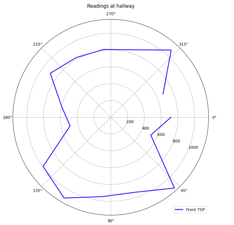
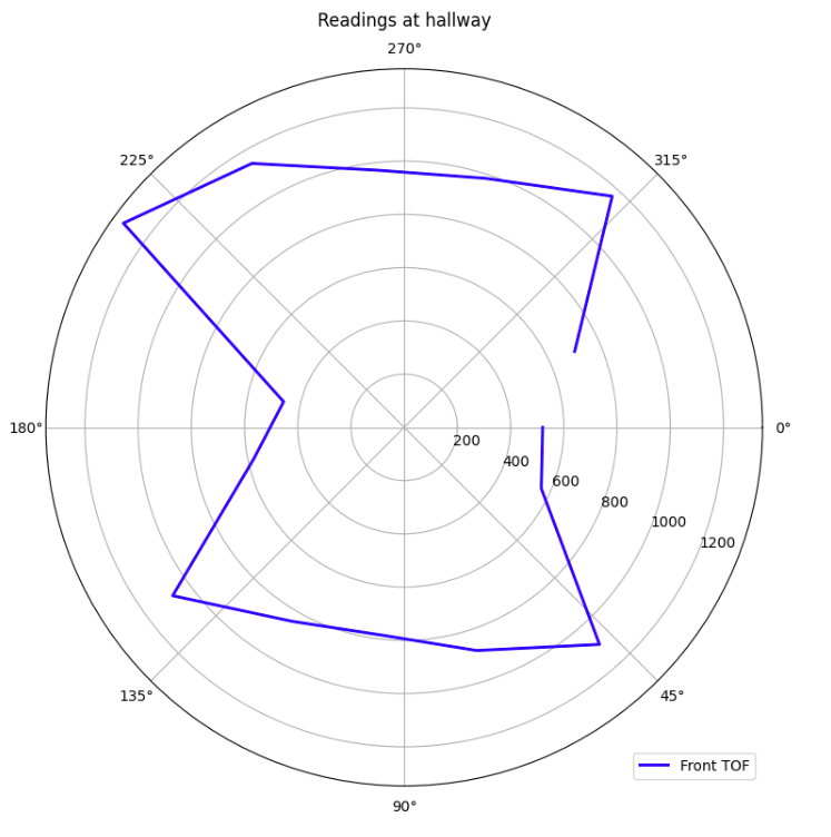
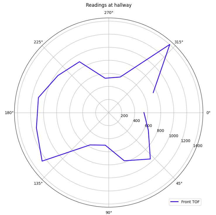
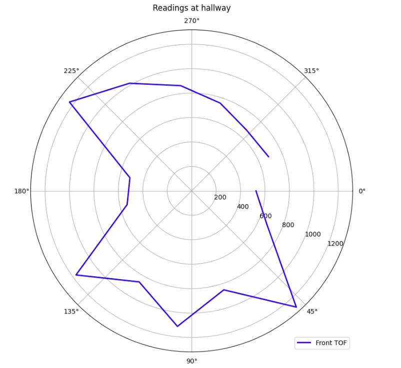
I placed the robot at 4 different positions in the hallway and recorded the data at these locations. For each
location I plotted the ToF vs yaw values on a polar plot. I have attached a photo of the hallway in which I did
the readings below. The polar coordinates graphs for Location 1 through Location 4 of the hallway are also shown
below.
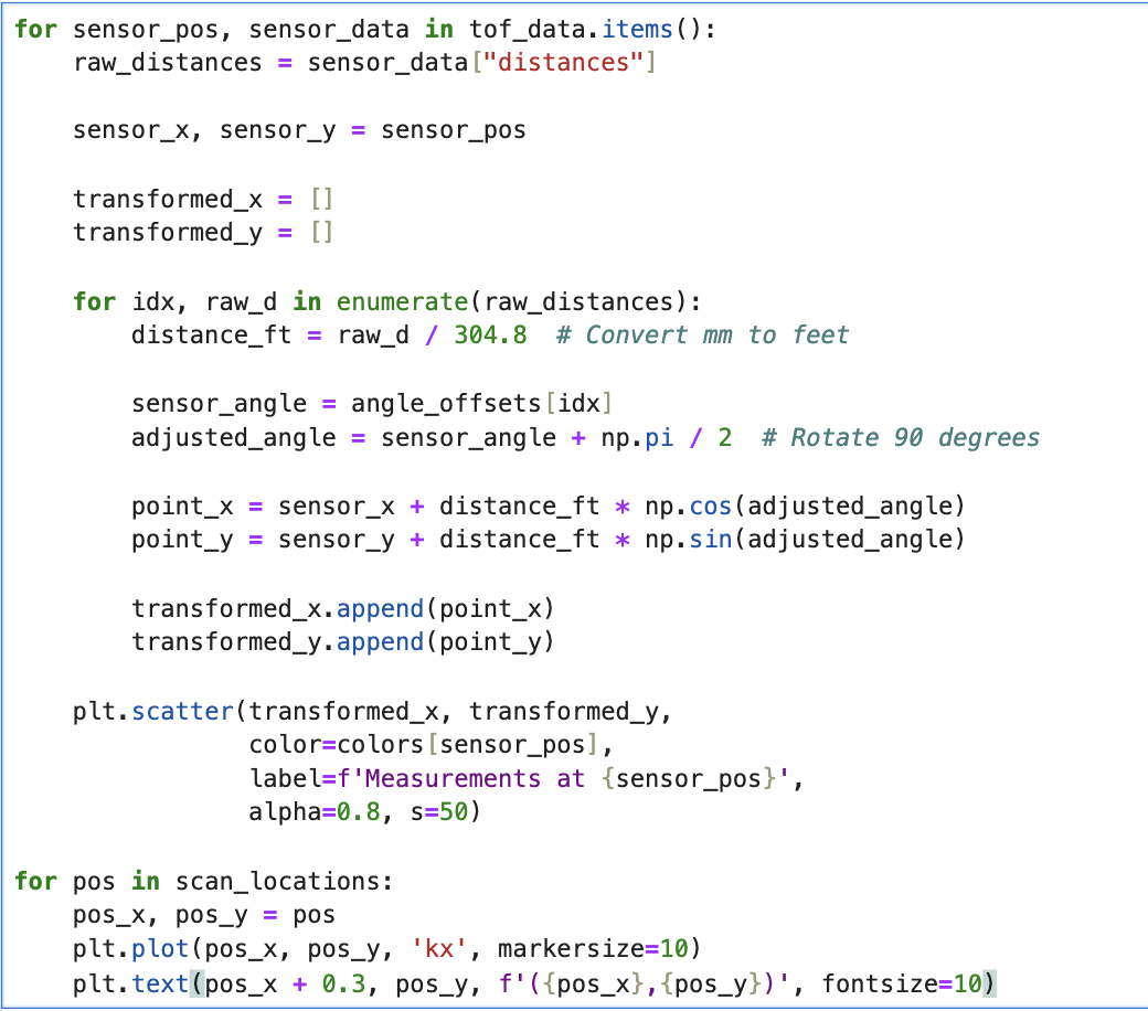
Once I had generated the four polar plots, for the next step I used the transformation matrices as described in
lecture to convert the polar plots to cartesian coordinates.
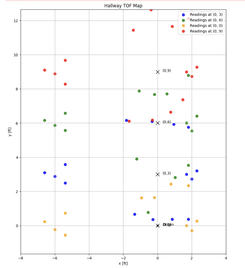
I had collected data from four positions in the hallways which I labeled as: (0, 0), (0, 3), (0, 6), and (0, 9)
feet and
used mathematical transformations to convert these raw distance readings into a coherent spatial map. The
algorithm applies different transformations based on the angle of each reading – points that should form the left
wall are placed farther out (around 6 feet) while the right wall points are positioned closer (about 2 feet),
creating an asymmetric hallway with more space on the left side.
Transformation Mathematics
The transformation from polar to Cartesian coordinates involves two main
steps:
1. Convert Polar to Local Cartesian Coordinates
Given a point in polar coordinates (r, θ), the local Cartesian coordinates are:
xlocal = r · cos(θ) ylocal = r · sin(θ)
2. Transform Local to Global Map Coordinates
Apply a transformation matrix to convert local coordinates to global coordinates using the robot's position and
orientation (xrobot, yrobot, α):
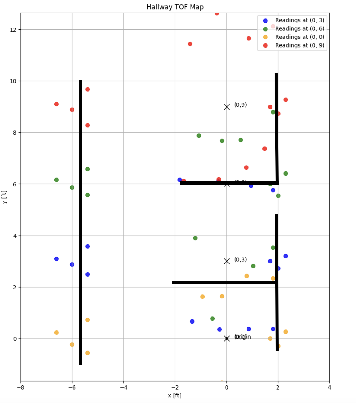
Once this was done I got the following map representing the hallway. I added in lines to the map based on the
hallway and got the below visualizations.
Conclusion
Overall, this lab provided valuable insights into robotic mapping techniques. By implementing a PID controller for
orientation control and collecting TOF sensor readings, I was able to successfully generate a
spatial representation of a hallway. I also was able to gain a better understanding of polar coordinates and
transformation matrices.
References
I referenced Stephan Wagner work for Lab 8. Further, Jennie Redrovan, Lulu Htutt, Daniela, Henry and I worked
on
this lab together and collaborated while figuring out the Kalman Filter implementation. Aidan Derocher was also
very helpful with debugging some issues.