The purpose of Lab 2, was to get familiar with the IMU and working with accelerometer and gyroscope data.
Lab Set-up
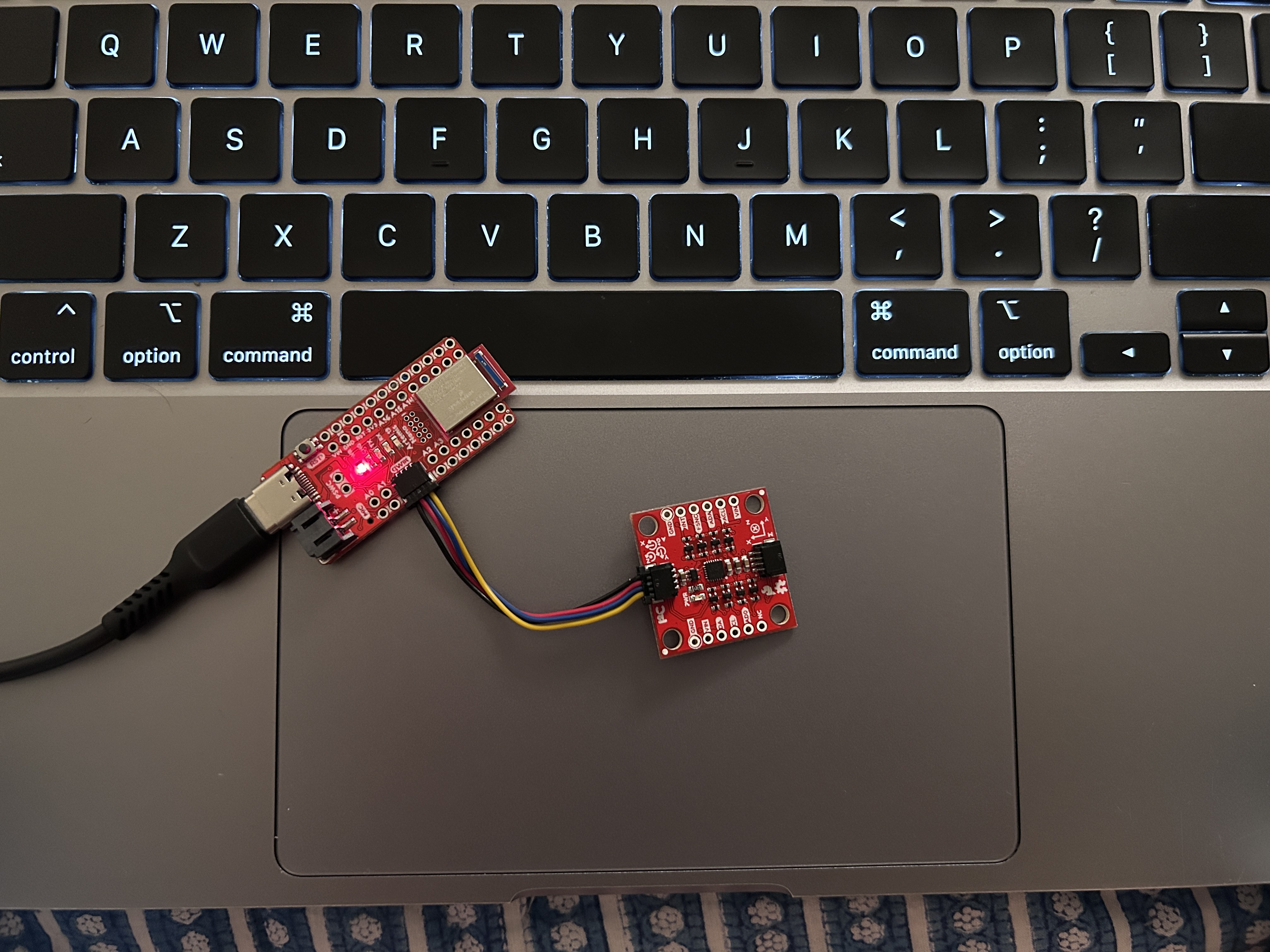
To set-up the lab I first downloaded the SparkFun 9DoF IMU Breakout - ICM 20948 Arduino library. I then connected
the IMU directly with the Artemis using a QWIIC cable connector. I also made sure to use the I2C port on the IMU.
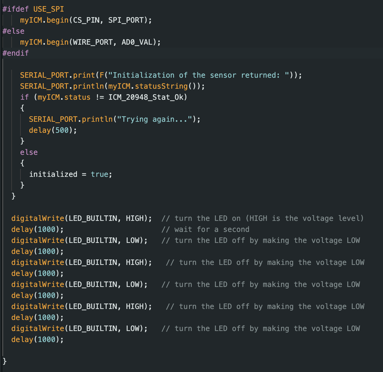
To ensure that the IMU is correctly communicating, I ran the Example1_Basics and checked the serial monitor
output. The ADO_VAL is the value of the last bit of the I2C address. The default value
is 1 and represents that the ADR jumper is open, and 0 represents that it is closed. Since our jumper is closed,
we set the value to the default of 1.
LED Blinking
As a visual indication that the IMU is running, I blinked the LED on board the Artemis 3 times on
initialization. As can be seen in the video, once the code is uploaded to the board, the LED blinks thrice
before we see any IMU output.
Analyzing Accelerometer Data
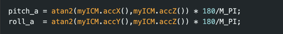
The accelerometer on the IMU measures data in X, Y, Z coordinates. To get the pitch and roll data, we have to
perform geometric transformations on the X, Y data. As described in lecture, we use the atan2 function to
convert the data using the following formula:
I then verified the IMU measurements when held at -90/0/90 degrees. Some of these readings are shown below.
It was a little hard to get exact readings, particularly close to 90 and -90 degrees. I was also unable to hold
the IMU completely still to get accurate readings.
To check the accuracy of the accelerometer and find an
appropriate conversion factor, I performed two point calibration:
Roll:
Reference range: 90 - (-90) = 180
Raw range = -89.27 - (-89.23) = 178.5
Corrected Value = 90.5
Pitch:
Reference range: 90 - (-90) = 180
Raw range = 90.23 - (-89.99) = 180.22
Corrected Value = 89.3
Filtering and FFTs
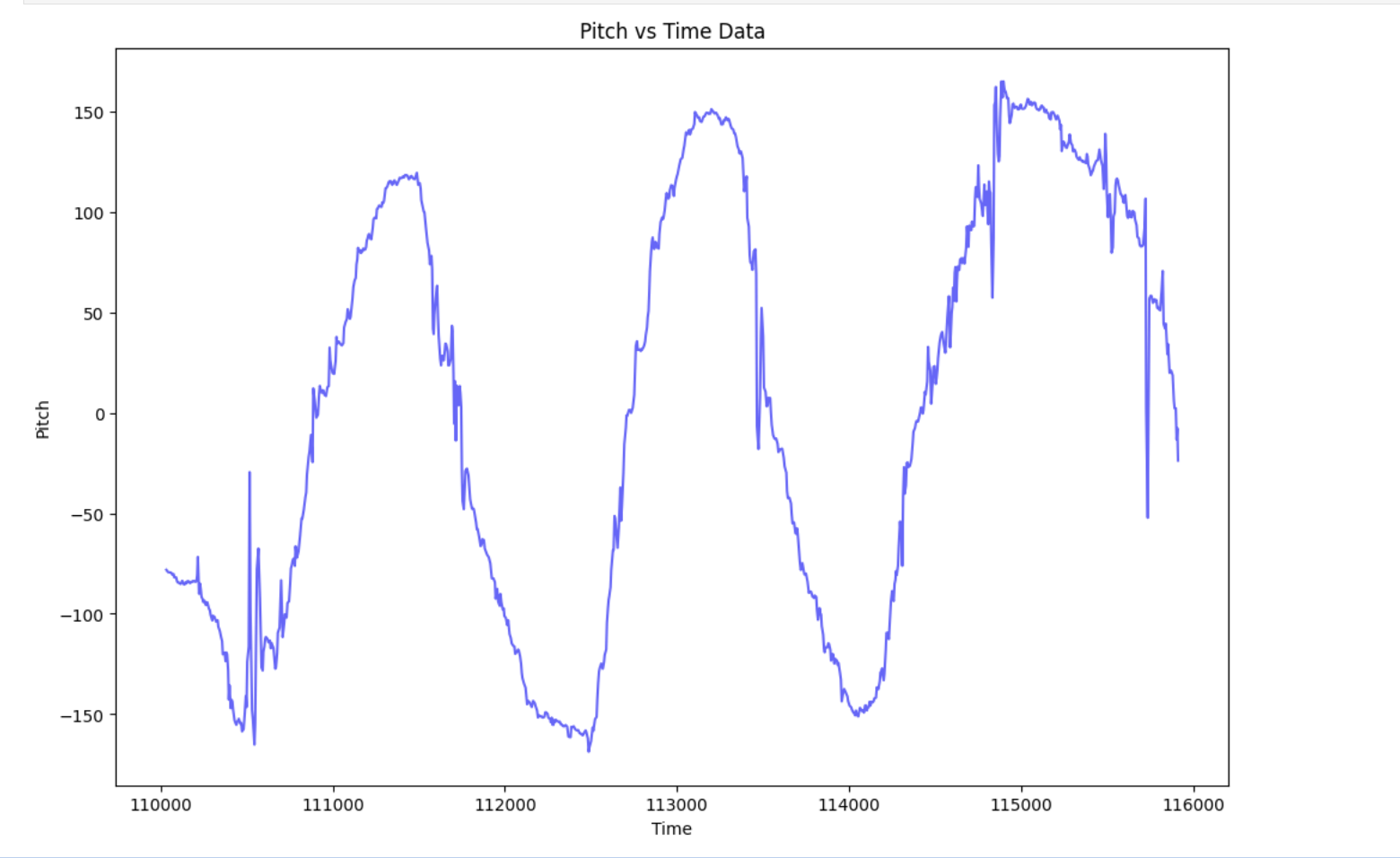
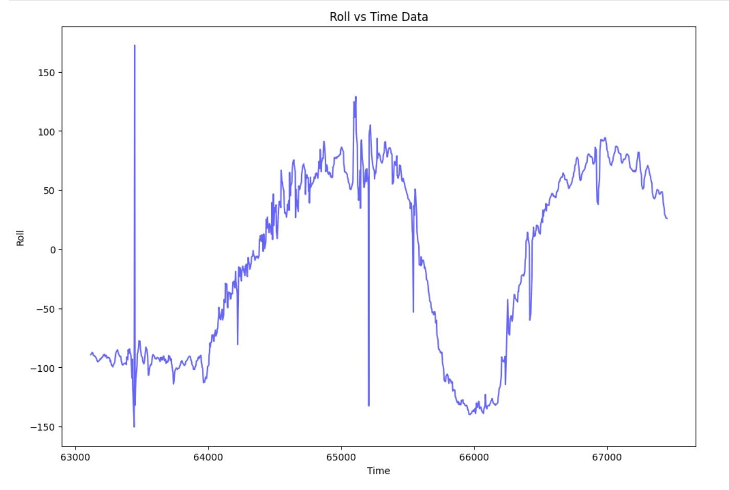
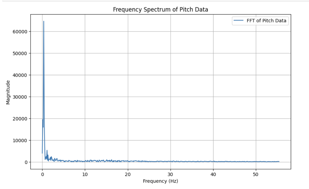
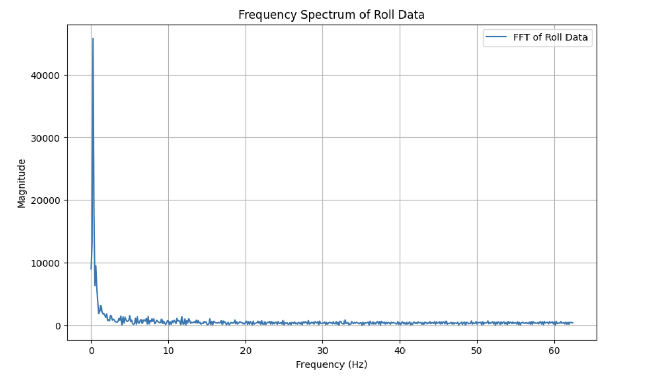
The accelerometer data had quite a lot of noise. To find an appropriate cut-off frequency for a low-pass filter,
I performed an FFT on the roll and pitch data respectively. I obtained this data by moving the IMU in such a way
as to get an approximate sine curve as reflected in the graphs below.
From the FFT, a reasonable cut-off frequency seems to be around 2-5Hz, i.e. most of our frequencies seem to be
concentrated in this range.
To find \( \alpha \), I used the following formula:
\[
\alpha = \frac{dt}{dt + RC}
\]
From these calculations I get \( \alpha \) = 0.12. I then implemented a low-pass filter as described in
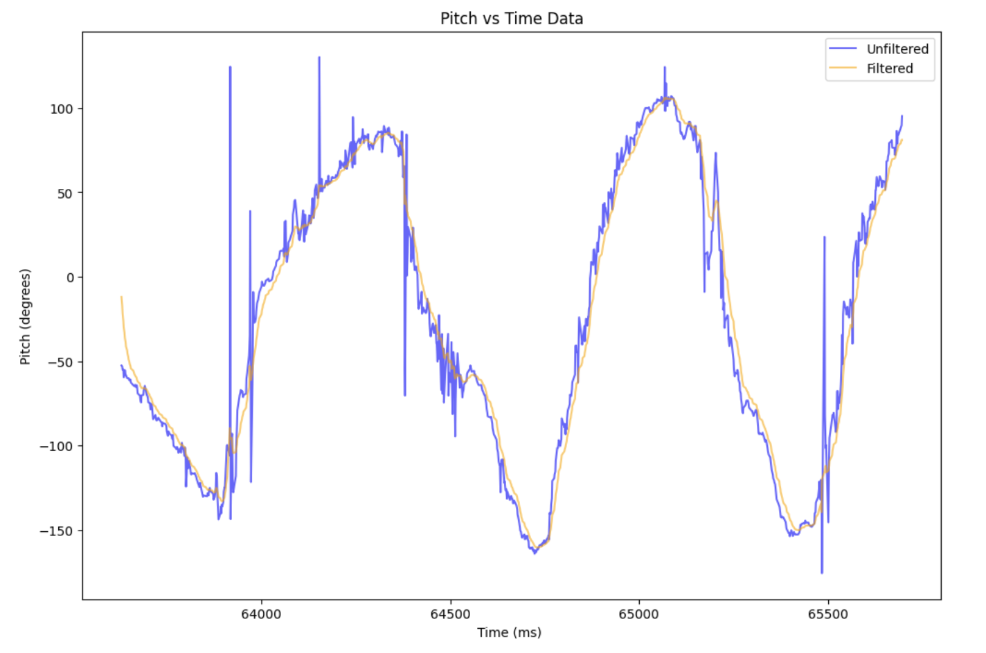
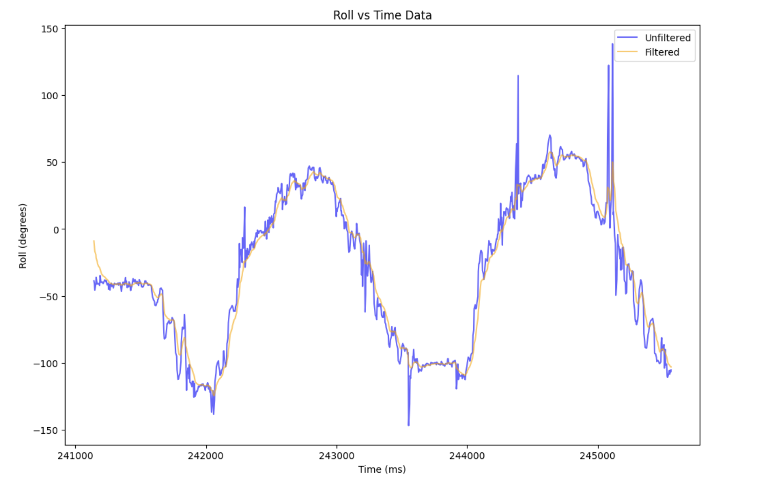
lecture using the following formula for the pitch and roll data. The data I used for this analysis was obtained
in a similar method as before, with some vibrational noise as well.
The graphs below show the difference in the filtered vs unfiltered data. As can be seen, the filtered data has a
noticeable reduction in noise while maintaining the shape of the unfiltered data. These graphs also show that
the calculated \( \alpha \) value is probably accurate for this problem.
Gyroscope
Next, we worked on the Gyroscope and calculated pitch, roll as well as yaw data. The accelerometer provided does
not calculate yaw data so we must obtain this from the gryroscope itself. Again, the gyroscope provides X, Y, Z
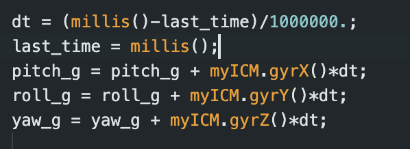
transitional data. To obtain the required rotational data, I used the formulas as described in lecture.
The gyroscope provides rads/s data which must be converted to degrees. Here, dt acts as an integration variable
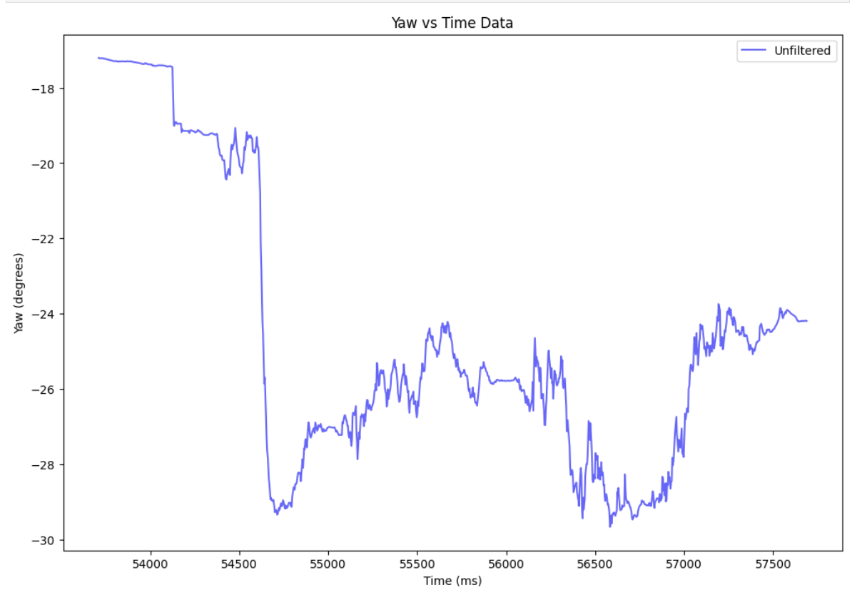
for the data. The gyroscoope data had much lesser noise than the accelerometer data on board, but also showed
some drift. The graphs for yaw data is shown below. Increasing the sampling frequency of the data seemed to lead
to more drift in the gryroscope data but almost the same amount of noise in the accelerometer data.
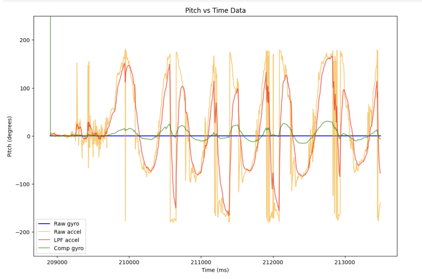
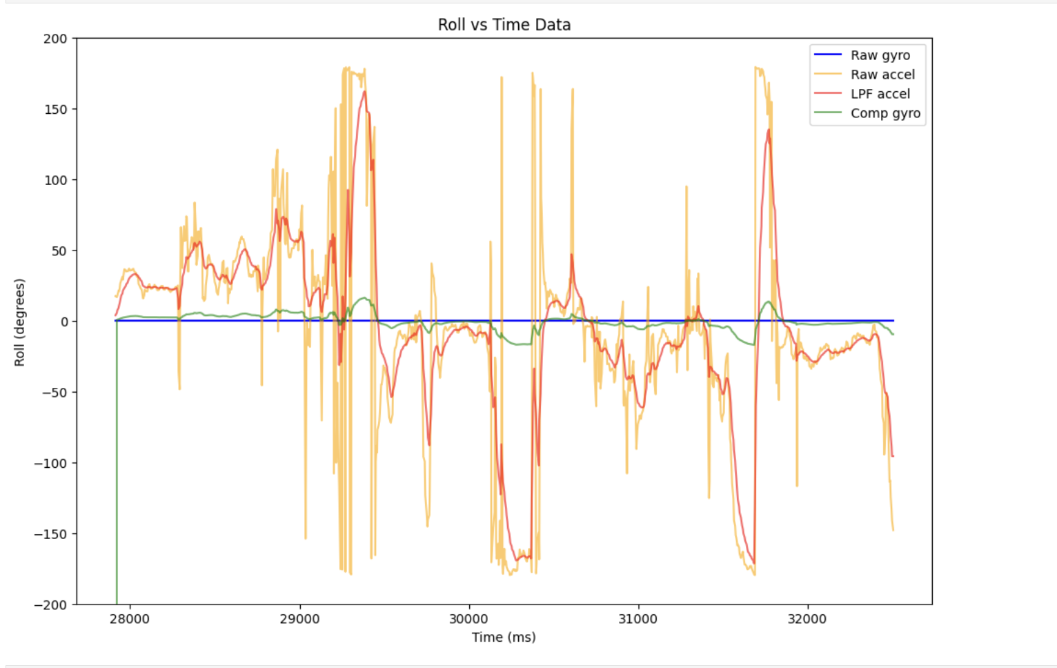
Complementary Filtering
Since the gyroscope data has some drift and the accelerometer data has noise, we can use a complementary filter
to combine the data from the two to get a more accurate reading of pitch and roll. For this filter, I used the
equations shown in class and used \( \alpha \) = 0.9 initially. I did this since the accelerometer data showed
higher accuracy.
The graphs below shows the raw and filtered accelerometer and gyroscope data.
Speed/Sampling Data
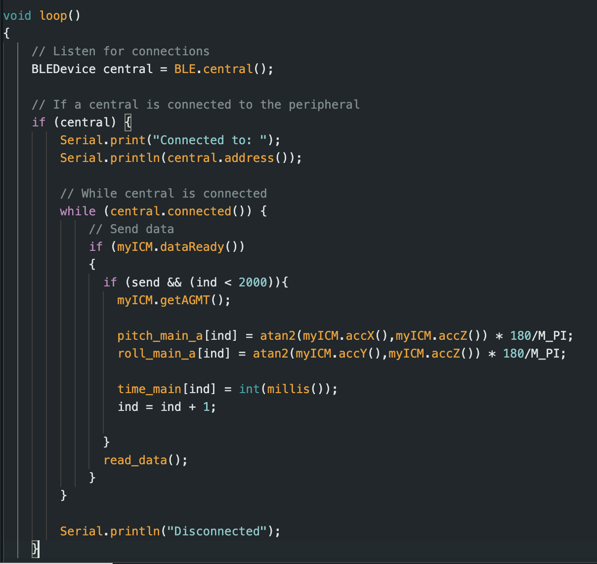
This task focused on speeding up data acquisition and sending/receiving process. My main loop in my arduino code
that was sending the data had a bunch of Serial.print statements which I removed. Further, I first stored all
the data in global arrays and then sent all the data over in bulk. I also added checks in the main loop to see
if the data is ready, and store it in the global arrays when it is. I store the pitch, roll and yaw data as
floats which my Python code separates and stores in different arrays. Floats have lesser overhead than double
does and seemed to capture the required data variation. Ints would not contain the required number of decimal
points for this data. After adding all the suggested optimizations to my code, I was able to receive 1000 data
points in 2.6 seconds.
There are 384000 bytes on the Artemis and each float value takes up 4 bytes. Therefore, a total of 96,000 data
points can be stored. Since we will be sending accelerometer, gyroscope and ToF data, this is a total of 32,000
data points. Further, as calculated above my current sampling rate is approx 2.6 seconds. Therefore, 32000 data
points would take 83.2 seconds fill up the Artemis.
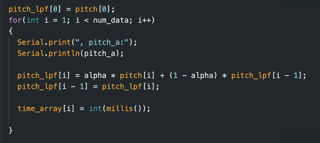
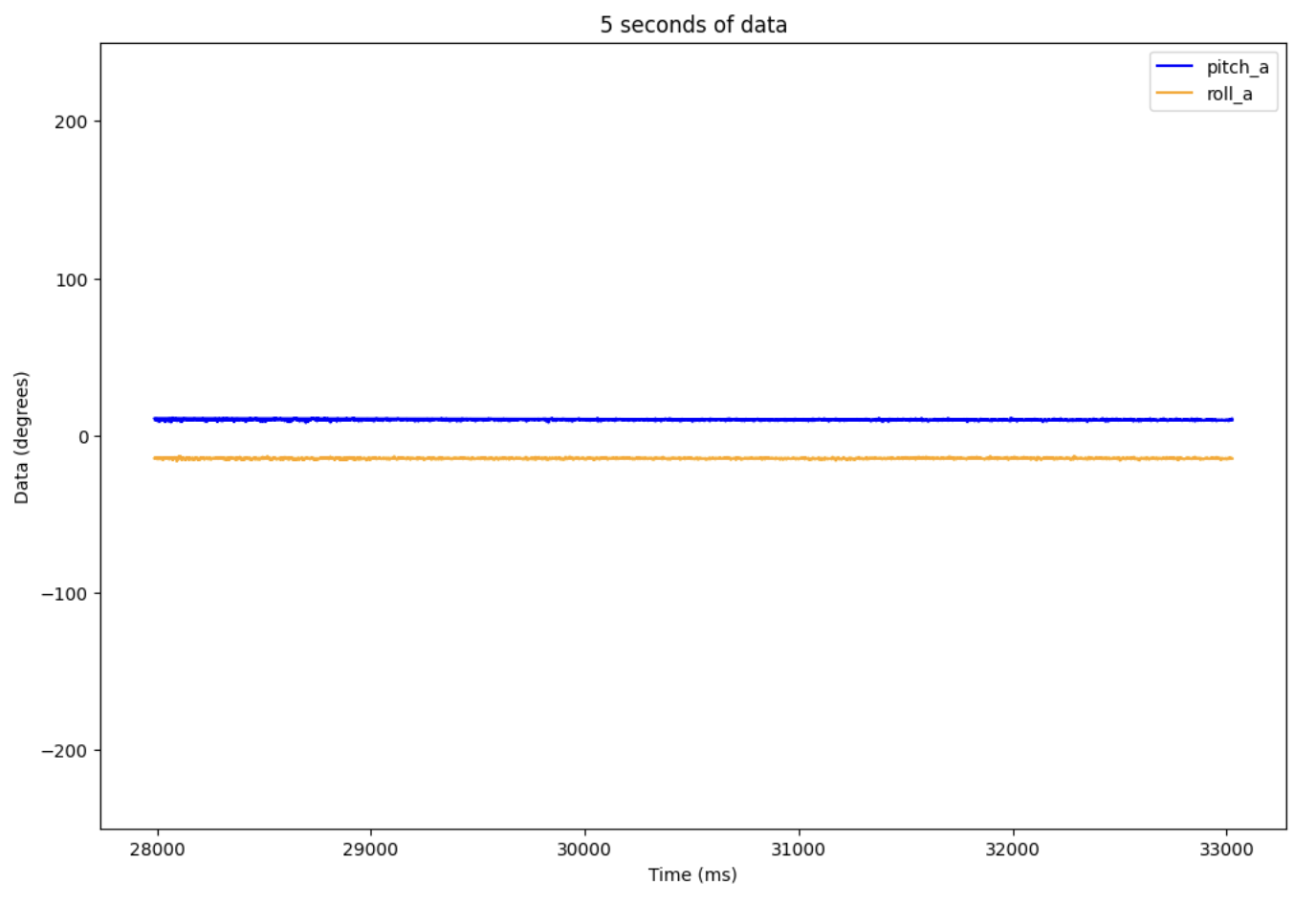
The above code shows how I collect 5 seconds of data in the main loop of the arduino code only when the send
flag is set to 1. The Python code receives these values and I have plotted them above.
Stunt
Lastly, I played around with the robot, running it around to understand how it works and how to get it to do a
stunt such as a flip.
Conclusion
This lab was very useful in getting familiar with working with IMU data and filters to reduce noise/drifting.
It also helped in reinforcing the different methods of interacting with and sending/receiving data between our
computer and the robot. This will
be
very useful in future labs where performance of the robot is crucial and it is important to pick the best method
of communication.
References
I used Nidhi Sonwalkar's lab report to check some of my steps. I also got the two-point calibration formula from
here. I also reference Daria's work for the last part.